Consensus Module Analysis

Introduction

In this vignette, we use Comethyl to construct a consensus weighted region comethylation network — a network built simultaneously across two biological groups (here, females and males) that share the same genomic region definitions. Because modules are identified jointly, any module that emerges represents comethylation structure that is reproducible across both groups rather than idiosyncratic to one.

The dataset used here is from the Babies GROWELL study (bgw_wgbs_comethyl), which investigates how prenatal family and community-level exposures influence early childhood DNA methylation, particularly in regions related to energy regulation and fat deposition. Children (ages 1–4) from mothers with pre-pregnancy BMI 25–40 were profiled by whole-genome bisulfite sequencing (WGBS). Females and males are analyzed as separate datasets using a shared region set so that modules can be compared directly between sexes. This is a test dataset which contains chr22 only. For learning the pipeline quickly, I highly recommend splitting your dataset into a smaller set of regions like chr22. Code used to generate this can be found here Make minidata for bgw_wgbs_comethyl

Relationship to other vignettes. The CpG Cluster Analysis and Gene Body Analysis vignettes document the single-dataset workflow. This vignette covers the multi-dataset extension. Many of the underlying comethyl functions are the same; the key differences are the reference region strategy, the joint SD filter (Script 05b), and the use of blockwiseConsensusModules() from WGCNA.

Environment Setup

All analyses should be run within the comethyl pixi environment to ensure reproducibility. If you have not yet set up the environment, see the Get Started vignette for full installation instructions.

Activate the environment before launching R:

# From the repository root
pixi shell       # activates the environment
R                # launch R from within it

# Or run scripts directly
pixi run Rscript scripts/consensus/00_import_cpg_reports_consensus.R --help

Setup

library(tidyverse)
library(comethyl)
library(WGCNA)
library(openxlsx)

Note on file paths. All file paths in this vignette are written relative to your project root — the top-level directory of your analysis (e.g., /path/to/my_project/). Before running any code, set your working directory to the project root:
setwd("/path/to/my_project")   # replace with your actual project root
getwd()                         # confirm before proceeding
The output directory tree (comethyl_output/consensus/) will be created automatically by each script. You do not need to create it manually.

Set Global Options

As in the single-dataset workflow, we disable WGCNA multi-threading when working with large region sets (> 150,000 regions). For smaller sets or interactive exploration you can enable threads with WGCNA::enableWGCNAThreads().

options(stringsAsFactors = FALSE)
Sys.setenv(R_THREADS = 1)
WGCNA::disableWGCNAThreads()

Overview of the Consensus Approach

The consensus workflow adds several steps before and after the steps you would recognise from the single-dataset vignettes. The overall logic is:

One reference dataset defines the canonical CpG filter and genomic regions. All other datasets must use exactly these regions.
Non-reference datasets are aligned to the reference CpG universe and their region methylation is calculated over the reference regions.
After all datasets have region methylation matrices, a shared region filter (Script 05b) keeps only regions that are present and sufficiently variable across both datasets.
PCs are derived and methylation is adjusted independently for each dataset (Scripts 06–07), with two adjustment strategies compared.
A single consensus soft-power is chosen that satisfies scale-free topology criteria in every dataset simultaneously (Script 08).
A soft-power benchmark (Script 08b) uses subsampled regions to efficiently compare power choices across adjustment versions, with Script 08c summarising results across all filter candidates.
blockwiseConsensusModules() identifies modules that are consistent across both sexes (Script 09).
Downstream analyses (diagnostics, membership, ME-trait correlations, annotation, enrichment) use the shared module assignments.

Choosing a Reference Dataset

The reference dataset determines which CpGs are retained and which genomic regions are defined. For sex-stratified analyses:

If you have a baseline or pre-treatment timepoint, this is usually the natural reference because it defines the methylation landscape before any intervention.
If you are comparing two biological groups (e.g. female vs. male), choose the group with the larger sample size or the group most central to your hypothesis as the reference.
If no single dataset is clearly primary, choose the one with the highest sequencing depth or most samples, as it will produce the most stable region definitions.
In the BGW analysis, females are used as the reference dataset.

Practical note. The reference only affects which CpGs and regions are defined in Scripts 01–02. Once regions are defined, all datasets are treated symmetrically in Script 05b onward.

Two Adjustment Strategies

Script 07 supports two adjustment modes that are compared throughout the downstream analysis:

Version	Description	When to use
`v1_all_pcs`	Regress out all top PCs	Simple baseline; conservative
`v2_exclude_protected_pcs`	Exclude PCs correlated with protected biological traits (e.g. sex, diagnosis)	When you want to preserve signal from key biological variables

Both versions are run in parallel and compared from Script 08 onward. Protected and technical traits are defined in config files (protected_traits.txt, technical_traits.txt). The only issue to be wary of is that the adjustments will be different based on the dataset. For instance, females might find no PCs associated with outcomes or exposures, while males find some variables associated with exposures or outcomes. So in v2, females will basically be v1, but for males v2 will actually be a true v2 because it adjusted out variation related to the PCs associated with key biological variables.

1. Import CpG Reports — Script 00

Run separately for each dataset (females and males).

getCpGs() reads Bismark CpG_report files into a single BSseq object and computes CpG totals at different coverage and per-sample cutoffs to guide filter choice. Run once per dataset — the cytosine reports for both sexes can live in the same directory since samples are matched via the metadata file.

Metadata File Format

The sample metadata file is an Excel spreadsheet read with openxlsx::read.xlsx(..., rowNames = TRUE). The first column must contain sample IDs that exactly match the Bismark CpG_report filenames (without the .CpG_report.txt.gz suffix). The first cell of row 1 (column A) should be left blank — this tells read.xlsx to treat that column as row names rather than a data column.

	Sex	Diagnosis	BMI	Age	Batch
Sample_01	0	1	28.4	32	1
Sample_02	1	0	31.2	29	1
Sample_03	0	1	26.7	35	2

All trait columns must be numeric. Categorical variables should be dummy-coded (e.g., Sex: F = 0, M = 1; Diagnosis: TD = 0, ASD = 1). Character values such as "Female", "<LOD", or blank cells will cause those columns to be silently dropped during downstream numeric filtering.

Common errors and fixes:

# Error: duplicate row names
# Cause: two samples share the same ID in column A
# Fix: ensure every sample has a unique identifier

# Error: no CpG report files found / sample mismatch
# Cause: row names don't match filenames in the cytosine report directory
# Check with:
list.files("data/processed/cytosine_reports/", pattern = "CpG_report")
rownames(colData_females)   # these must overlap

# Silent drop of trait columns (e.g. DDT, PCBs, sex)
# Cause: column contains "<LOD", "ND", blanks, or mixed types
# Fix: coerce to numeric before passing to the pipeline
colData_females <- colData_females %>%
  mutate(across(everything(), ~ suppressWarnings(as.numeric(as.character(.)))))

# ── Females (reference) ───────────────────────────────────────────────────────
colData_females <- openxlsx::read.xlsx("data/metadata/merged_qc_females.xlsx",
                                        rowNames = TRUE)
setwd("data/processed/cytosine_reports/")
bs_females_unfiltered <- getCpGs(
  colData = colData_females,
  file    = "comethyl_output/consensus/00_cpg_extraction/females/Unfiltered_BSseq.rds"
)
setwd("../../..")

CpGtotals_females <- getCpGtotals(
  bs_females_unfiltered,
  file = "comethyl_output/consensus/00_cpg_extraction/females/CpG_Totals.txt"
)
plotCpGtotals(CpGtotals_females,
              file = "comethyl_output/consensus/00_cpg_extraction/females/CpG_Totals.pdf")

# ── Males ─────────────────────────────────────────────────────────────────────
colData_males <- openxlsx::read.xlsx("data/metadata/merged_qc_males.xlsx",
                                      rowNames = TRUE)
setwd("data/processed/cytosine_reports/")
bs_males_unfiltered <- getCpGs(
  colData = colData_males,
  file    = "comethyl_output/consensus/00_cpg_extraction/males/Unfiltered_BSseq.rds"
)
setwd("../../..")

CpGtotals_males <- getCpGtotals(
  bs_males_unfiltered,
  file = "comethyl_output/consensus/00_cpg_extraction/males/CpG_Totals.txt"
)
plotCpGtotals(CpGtotals_males,
              file = "comethyl_output/consensus/00_cpg_extraction/males/CpG_Totals.pdf")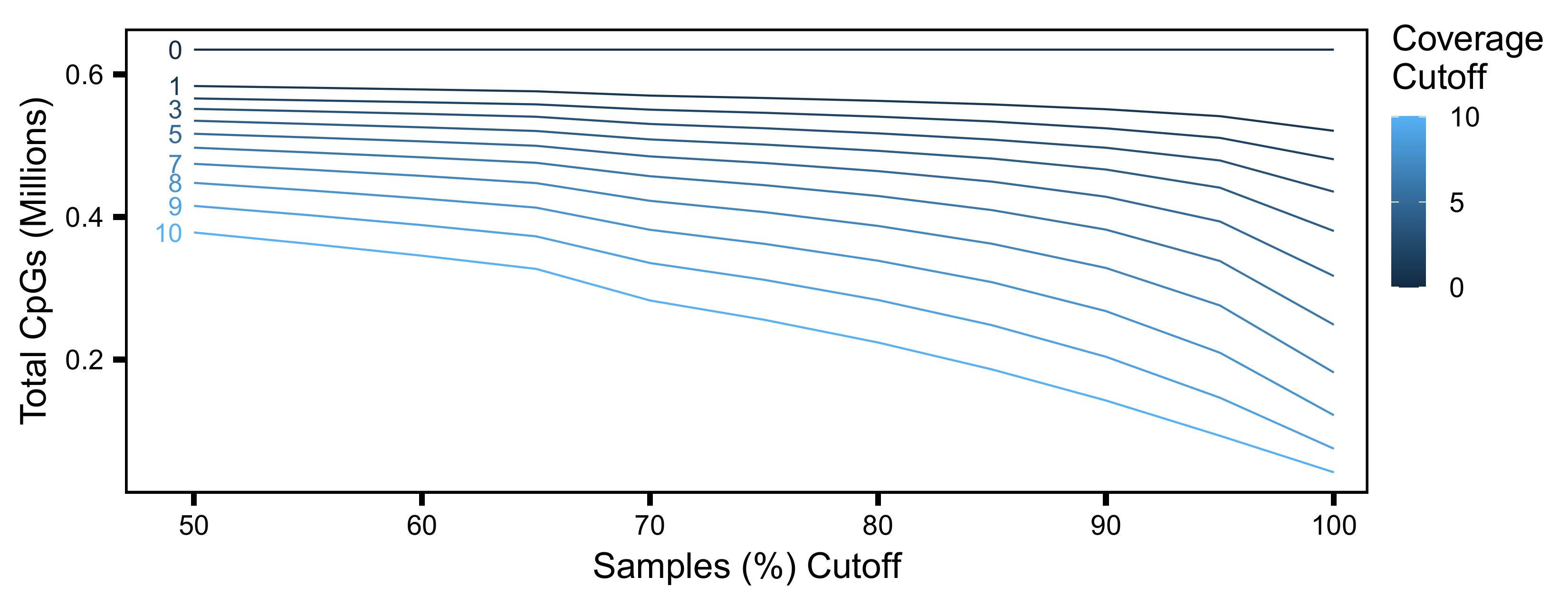

Figure 1. CpG Totals — Females

Figure 1. CpG totals for the female dataset across a range of coverage and per-sample cutoffs. Use this plot as well as CpG_Totals.txt to select a cov and perSample combination that retains a reasonable number of CpGs without sacrificing too many samples.

2. Filter CpGs and Define Reference Regions — Script 01

Run on the reference dataset (females) only.

filterCpGs() retains CpGs meeting minimum coverage and per-sample requirements. getRegions() then clusters retained CpGs into genomic regions. These regions are the canonical definitions reused by all other datasets. Here we keep CpGs with at least 3 reads in at least 75% of samples (cov = 3, perSample = 0.75).

bs_females <- filterCpGs(
  bs        = bs_females_unfiltered,
  cov       = 3,
  perSample = 0.75,
  file      = "comethyl_output/consensus/01_reference_filter_regions/females/cov3_75pct/Filtered_BSseq.rds"
)

regions_raw <- getRegions(
  bs   = bs_females,
  file = "comethyl_output/consensus/01_reference_filter_regions/females/cov3_75pct/Regions.txt"
)

plotRegionStats(regions_raw, maxQuantile = 0.99,
                file = "comethyl_output/consensus/01_reference_filter_regions/females/cov3_75pct/Region_Plots.pdf")
plotSDstats(regions_raw, maxQuantile = 0.99,
            file = "comethyl_output/consensus/01_reference_filter_regions/females/cov3_75pct/SD_Plots.pdf")

regionTotals <- getRegionTotals(
  regions_raw,
  file = "comethyl_output/consensus/01_reference_filter_regions/females/cov3_75pct/Region_Totals.txt"
)
plotRegionTotals(regionTotals,
                 file = "comethyl_output/consensus/01_reference_filter_regions/females/cov3_75pct/Region_Totals.pdf")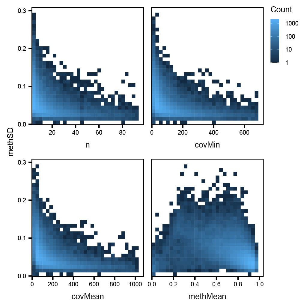

Figure 2. Unfiltered Region SD Plots — Females

Figure 2. Methylation standard deviation versus region statistics for unfiltered regions in the female dataset. Regions with low coverage tend to have high SD driven by technical noise rather than biology.

Figure 3. Region Totals — Females

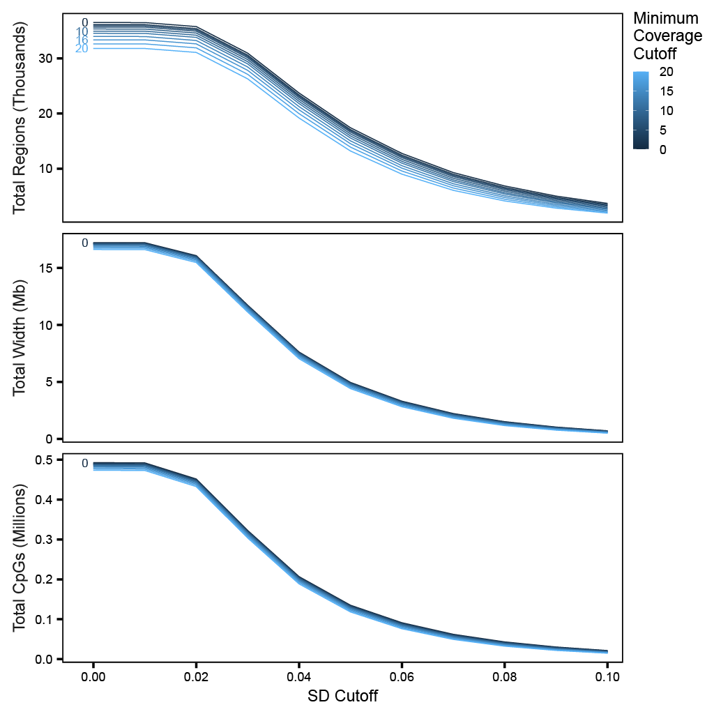
Figure 3. Number of regions remaining after filtering at different covMin and methSD combinations. Use this plot to choose thresholds before running Script 02.

3. Filter Reference Regions — Script 02

Run on the reference dataset (females) only.

filterRegions() applies minimum coverage (covMin) and methylation SD (methSD) thresholds to the raw regions.

Key design decision: set `methSD = 0` for sex-stratified analyses

For earlier analyses, regions were often defined using a single reference dataset. For example, we selected regions in females using covMin = 10 and methSD = 0.05, and then extracted the matching regions in males. This approach can work when the reference dataset captures the major sources of methylation variability. However, it can be problematic for sex-stratified analyses because a region that is variable in males may be nearly invariant in females, or vice versa. If a strict SD filter is applied only to the reference group, sex-specific variable regions may be discarded before the other group is evaluated.

Recommended approach for sex-stratified group comparisons: set methSD = 0 (or a very permissive value) in Script 02, set methSD = 0 and apply only the coverage prefilter, such as covMin = 10 in the BGW analysis. The decisive variability filter should then be applied later in Script 05b using both sex-specific datasets.

In Script 05b, the preferred SD filter is to retain regions with sufficient variability in either sex, for example SD ≥ 0.05 in females or SD ≥ 0.05 in males. This preserves regions that may be biologically informative in only one sex while still removing regions that are invariant in both groups.

# Coverage prefilter only — methSD = 0 is deliberate for sex-stratified design
regions_filtered <- filterRegions(
  regions = regions_raw,
  covMin  = 10,
  methSD  = 0,
  file    = "comethyl_output/consensus/02_reference_region_filter/females/cov3_75pct/covMin10_methSD0/Filtered_Regions.txt"
)

plotRegionStats(regions_filtered, maxQuantile = 0.99,
                file = "comethyl_output/consensus/02_reference_region_filter/females/cov3_75pct/covMin10_methSD0/Filtered_Region_Plots.pdf")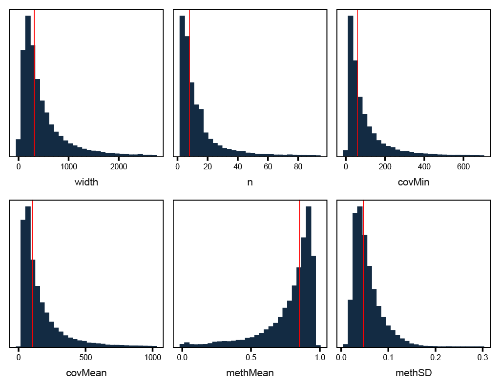

Figure 4. Filtered Region Plots — Females

Figure 4. Region statistics after applying the coverage prefilter (covMin = 10, methSD = 0). No SD filter is applied at this stage — that happens jointly in Script 05b.

4. Build Reference Region Methylation — Script 03

Run on the reference dataset (females) only.

getRegionMeth() calculates region-level percent methylation from the filtered BSseq object using the canonical reference regions from Script 02.

meth_females_raw <- getRegionMeth(
  regions = regions_filtered,
  bs      = bs_females,
  file    = "comethyl_output/consensus/03_region_methylation/females/cov3_75pct/covMin10_methSD0/Region_Methylation.rds"
)

5. Align Other Datasets to Reference CpGs — Script 04

Run on non-reference datasets (males) only.

The male CpG_report files are restricted to the CpG universe of the female filtered BSseq using subsetByOverlaps(). A permissive filter (cov = 3, perSample = 0.75) is then applied to remove any remaining low-coverage CpGs from the aligned object.

bs_females_filtered <- readRDS(
  "comethyl_output/consensus/01_reference_filter_regions/females/cov3_75pct/Filtered_BSseq.rds"
)

setwd("data/processed/cytosine_reports/")
bs_males_unfiltered <- getCpGs(
  colData = colData_males,
  file    = "comethyl_output/consensus/04_align_to_reference_cpgs/males/Unfiltered_BSseq.rds"
)
setwd("../../..")

# Restrict males to the reference (female) CpG universe
bs_males_aligned <- subsetByOverlaps(bs_males_unfiltered, bs_females_filtered)

bs_males_aligned <- filterCpGs(
  bs        = bs_males_aligned,
  cov       = 3,
  perSample = 0.75,
  file      = "comethyl_output/consensus/04_align_to_reference_cpgs/males/Filtered_BSseq.rds"
)

6. Build Male Region Methylation — Script 05

Run on non-reference datasets (males) only.

Region methylation is calculated for males using the same canonical reference regions from Script 02. This ensures both datasets have methylation matrices over identical regions.

meth_males_raw <- getRegionMeth(
  regions = regions_filtered,
  bs      = bs_males_aligned,
  file    = "comethyl_output/consensus/03_region_methylation/males/cov3_75pct/covMin10_methSD0/Region_Methylation.rds"
)

7. Filter Shared, Complete Regions — Script 05b

This step is unique to the consensus workflow and is where the decisive variability filter is applied. It identifies regions that are complete (no missing values) and sufficiently variable in both datasets to build a good network.

Selection modes

Mode	Description	When to use
`complete_only`	Present and NA-free in every dataset	Legacy / simple case
`joint_sd_all`	Complete AND SD ≥ threshold in every dataset	Recommended for sex-stratified analyses
`joint_sd_any`	Complete AND SD ≥ threshold in at least one dataset	Discovery; may retain low-variability regions in some groups
`joint_sd_min_n`	Complete AND SD ≥ threshold in at least N datasets	Flexible middle ground for 3+ datasets

Recommended SD value. A threshold of joint_meth_sd = 0.05 (5% methylation SD) is used in the BGW analysis. This ensures every retained region has enough biological variability to contribute meaningful signal in both females and males. Examine the per-region SD distribution from Script 01 to calibrate for your data — the --write_sd_table TRUE flag outputs per-region SD diagnostics to help.

meth_females_raw <- readRDS(
  "comethyl_output/consensus/03_region_methylation/females/cov3_75pct/covMin10_methSD0/Region_Methylation.rds"
)
meth_males_raw <- readRDS(
  "comethyl_output/consensus/03_region_methylation/males/cov3_75pct/covMin10_methSD0/Region_Methylation.rds"
)

# Shared complete regions (joint_sd_all mode)
joint_meth_sd <- 0.05
shared_regions <- intersect(rownames(meth_females_raw), rownames(meth_males_raw))

meth_f <- meth_females_raw[shared_regions, ]
meth_m <- meth_males_raw[shared_regions, ]

sd_f <- apply(meth_f, 1, sd, na.rm = TRUE)
sd_m <- apply(meth_m, 1, sd, na.rm = TRUE)

pass <- (sd_f >= joint_meth_sd) & (sd_m >= joint_meth_sd)
message("Regions passing joint SD filter: ", sum(pass), " of ", length(pass))

meth_females_final <- meth_f[pass, ]
meth_males_final   <- meth_m[pass, ]

saveRDS(meth_females_final,
        "comethyl_output/consensus/05b_shared_complete_regions/cov3_75pct/covMin10_methSD0_jointSDall0p05/females_Methylation_jointEligible.rds")
saveRDS(meth_males_final,
        "comethyl_output/consensus/05b_shared_complete_regions/cov3_75pct/covMin10_methSD0_jointSDall0p05/males_Methylation_jointEligible.rds")

Figure 5. Joint SD Filter Summary

Figure 5. Per-region methylation SD distributions for females and males before and after the joint SD filter (joint_meth_sd = 0.05). Regions below the threshold in either group are removed.

8. PC Diagnostics — Script 06

Run separately for each dataset.

getPCs() derives principal components for each dataset. The PC-trait correlation heatmaps produced by Script 06 guide the choice of which PCs to include in the methylation adjustment. Protected biological traits (e.g., child sex, diagnosis) are defined in separate config files to inform the v2 adjustment strategy.

mod_females <- model.matrix(~1, data = pData(bs_females))
PCs_females <- getPCs(
  meth = meth_females_final,
  mod  = mod_females,
  file = "comethyl_output/consensus/06_pc_diagnostics/females/cov3_75pct/covMin10_methSD0_jointSDall0p05/PCs.rds"
)

# Examine PC-trait correlations to guide adjustment choice
# Saved to: 06_pc_diagnostics/females/.../PC_Trait_Correlation_Stats_Bicor.tsv

mod_males <- model.matrix(~1, data = pData(bs_males_aligned))
PCs_males <- getPCs(
  meth = meth_males_final,
  mod  = mod_males,
  file = "comethyl_output/consensus/06_pc_diagnostics/males/cov3_75pct/covMin10_methSD0_jointSDall0p05/PCs.rds"
)

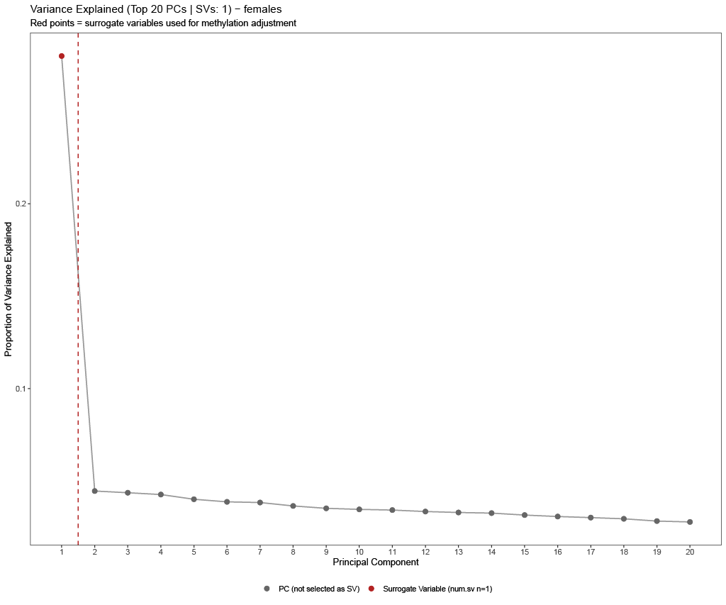
Figure 6. PC Variance Explained — Females

Figure 6. Variance explained by the top 20 PCs for the female dataset. The scree plot helps identify how many PCs to include in the adjustment. The PCs in red are what is considered a surrogate variable (SV). For females, only 1 PC was considered an SV

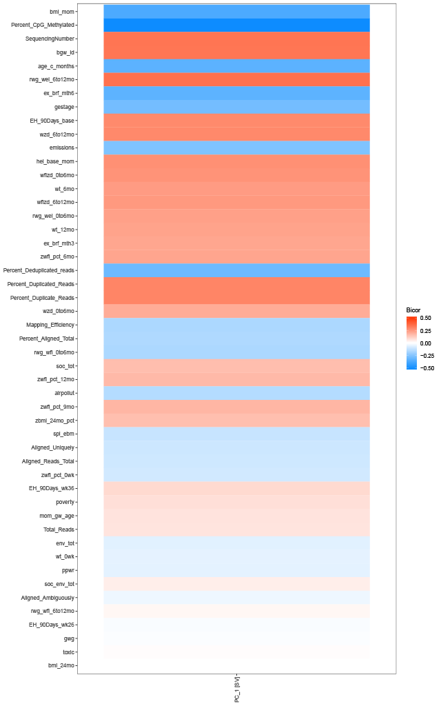
Figure 7. PC-Trait Correlation Heatmap — Females

Figure 7. Bicor correlations between PCs and sample traits for the female dataset. PCs associated with technical covariates (e.g. coverage, batch) are candidates for inclusion in the adjustment model.

Figure 8. PC Variance Explained — Males

Figure 8. Variance explained by the top 20 PCs for the male dataset. The scree plot helps identify how many PCs to include in the adjustment. The PCs in red are what is considered a surrogate variable (SV). For males, only 3 PC was considered an SV. The ones associated with variables were protected from adjustment.

Figure 9. PC-Trait Correlation Heatmap — Males

Figure 9. Bicor correlations between PCs and sample traits for the male dataset. PCs associated with technical covariates (e.g. coverage, batch) are candidates for inclusion in the adjustment model.

9. Adjust Methylation — Script 07

Run separately for each dataset.

adjustRegionMeth() regresses selected PCs out of the region methylation matrix. Two versions are run and compared:

v1 (all PCs): regress out all top PCs. Simplest approach; may inadvertently remove biological signal if a PC captures both technical and biological variance.
v2 (exclude protected PCs): exclude PCs significantly correlated (p < 0.05, bicor) with protected traits such as child sex or diagnosis. This preserves biological signal while removing technical confounders.

# ── v1: all PCs ───────────────────────────────────────────────────────────────
methAdj_females_v1 <- adjustRegionMeth(
  meth = meth_females_final,
  PCs  = PCs_females,
  file = "comethyl_output/consensus/07_methylation_adjustment/females/cov3_75pct/covMin10_methSD0_jointSDall0p05/v1_all_pcs/females_Adjusted_Region_Methylation_allPCs.rds"
)

# ── v2: exclude protected PCs ─────────────────────────────────────────────────
# Protected traits loaded from config/protected_traits.txt
methAdj_females_v2 <- adjustRegionMeth(
  meth = meth_females_final,
  PCs  = PCs_females,
  file = "comethyl_output/consensus/07_methylation_adjustment/females/cov3_75pct/covMin10_methSD0_jointSDall0p05/v2_exclude_protected_pcs/females_Adjusted_Region_Methylation_excluding_protected_PCs_bicor.rds"
)

# Repeat v1 and v2 for males ...

Figure 8. Sample Dendrogram After Adjustment — Females v1

Figure 8. Sample dendrogram based on adjusted region methylation (v1, all PCs) for the female dataset. Samples should no longer cluster strongly by technical batch after adjustment.

10. Select Consensus Soft Power — Script 08

getSoftPower() analyses scale-free topology for each dataset separately across a range of soft-thresholding powers. A single shared consensus power must then be chosen — the lowest power where R² ≥ 0.8 and the slope is negative in both females and males simultaneously. Using a shared power is essential: it ensures the network analysis is directly comparable across datasets.

sft_females <- getSoftPower(
  methAdj_females_v1,
  corType = "pearson",
  file    = "comethyl_output/consensus/08_soft_power/females/cov3_75pct/covMin10_methSD0_jointSDall0p05/v1_all_pcs/SoftPower_pearson.rds"
)
sft_males <- getSoftPower(
  methAdj_males_v1,
  corType = "pearson",
  file    = "comethyl_output/consensus/08_soft_power/males/cov3_75pct/covMin10_methSD0_jointSDall0p05/v1_all_pcs/SoftPower_pearson.rds"
)

plotSoftPower(sft_females,
              file = "comethyl_output/consensus/08_soft_power/females/cov3_75pct/covMin10_methSD0_jointSDall0p05/v1_all_pcs/SoftPower_Plots.pdf")
plotSoftPower(sft_males,
              file = "comethyl_output/consensus/08_soft_power/males/cov3_75pct/covMin10_methSD0_jointSDall0p05/v1_all_pcs/SoftPower_Plots.pdf")

Examine both plots side by side and identify the lowest power where both datasets cross R² = 0.8 with a negative slope. If the two datasets cross at different powers, use the higher of the two values so that scale-free topology is satisfied in both.

# After examining the plots, set the chosen power manually
chosen_power <- 12   # update based on your soft power plots
message("Chosen consensus soft power: ", chosen_power)

Figure 9. Soft Power Plots — Females

Figure 9. Scale-free topology fit (R²) and mean connectivity across soft power values for the female dataset. Select the lowest power where R² ≥ 0.8 with a negative slope.

Figure 10. Soft Power Plots — Males

Figure 10. Scale-free topology fit (R²) and mean connectivity for the male dataset. The consensus power must satisfy R² ≥ 0.8 in both datasets — use the higher of the two crossing points if they differ.

Optional: Soft-Power Benchmark — Scripts 08b and 08c

This step is optional. For large datasets where running getSoftPower() on the full region set is computationally expensive, Script 08b provides a faster alternative using a subsampled region set. If you have already run Script 08 above and are satisfied with the chosen power, you can skip to Script 09.

Script 08b runs soft-power analysis on a random subsample of regions across multiple seeds and adjustment versions, giving a quick estimate of the likely consensus power without the full computational cost. Script 08c then compares results across all region-filter candidates in a single summary, which is useful when testing multiple covMin or joint_meth_sd combinations.

Key parameters:

subsample_size: number of regions per seed (2,000 in BGW) — large enough to be representative, small enough to run in minutes.
n_seeds: seeds to average over (5 in BGW), reducing the impact of any single subsample.
scale_free_cutoff: R² threshold (0.8 is standard).

# Script 08b is run via command line. The interactive equivalent
# for examining results after the run:

sft_summary <- read.table(
  "comethyl_output/consensus/08b_softpower_benchmark/shared/cov3_75pct/covMin10_methSD0_jointSDall0p05/v1_all_pcs/subsample2000/combined_softpower_summary.tsv",
  header = TRUE, sep = "\t"
)

chosen_power <- read.table(
  "comethyl_output/consensus/08b_softpower_benchmark/shared/cov3_75pct/covMin10_methSD0_jointSDall0p05/v1_all_pcs/subsample2000/chosen_power.txt"
)$V1

message("Chosen consensus soft power from benchmark (v1): ", chosen_power)

Figure 11. Soft Power Benchmark Comparison — Script 08c

Figure 11. Summary of soft-power benchmark results across region filter candidates and adjustment versions (Script 08c). Use this to confirm that the chosen power is consistent across different filter choices. .*

11. Identify Consensus Modules — Script 09

blockwiseConsensusModules() identifies comethylation modules that are consistent across both females and males. Two versions are run (v1 and v2 adjustment) and compared.

Key arguments:

power: the consensus soft power selected in Script 08b.
consensus_cor: "pearson" (used in BGW) for higher sensitivity.
deep_split: module detection sensitivity 0–4; 4 gives more, smaller modules.
min_module_size: minimum regions per module (50 in BGW); increase to reduce very small modules.
merge_cut_height: modules with eigengene correlation above this threshold are merged (0.2 in BGW); lower values produce fewer, broader modules.
network_calibration: "single quantile" is used in BGW.

# Load final adjusted methylation matrices (v1 shown; repeat for v2)
methAdj_females_v1 <- readRDS(
  "comethyl_output/consensus/07_methylation_adjustment/females/cov3_75pct/covMin10_methSD0_jointSDall0p05/v1_all_pcs/females_Adjusted_Region_Methylation_allPCs.rds"
)
methAdj_males_v1 <- readRDS(
  "comethyl_output/consensus/07_methylation_adjustment/males/cov3_75pct/covMin10_methSD0_jointSDall0p05/v1_all_pcs/males_Adjusted_Region_Methylation_allPCs.rds"
)

multiExpr <- list(
  females = list(data = t(methAdj_females_v1)),
  males   = list(data = t(methAdj_males_v1))
)

consensus_modules <- blockwiseConsensusModules(
  multiExpr          = multiExpr,
  power              = chosen_power,
  corType            = "pearson",
  networkType        = "signed",
  TOMType            = "signed",
  deepSplit          = 4,
  minModuleSize      = 50,
  mergeCutHeight     = 0.2,
  maxBlockSize       = 40000,
  networkCalibration = "single quantile",
  saveTOMs           = TRUE,
  numericLabels      = FALSE,
  verbose            = 3
)

saveRDS(consensus_modules,
        "comethyl_output/consensus/09_consensus_modules/shared/cov3_75pct/covMin10_methSD0_jointSDall0p05/v1_all_pcs/Consensus_Modules.rds")

module_colors <- consensus_modules$colors
message("Modules detected: ", length(unique(module_colors[module_colors != "grey"])))
table(module_colors)

Figure 12. Region Dendrograms — v1

Figure 12. Region dendrograms with consensus module color assignments (v1 adjustment). Each color represents a module of comethylated regions shared between females and males.

12. Consensus Module Diagnostics — Script 10

After module detection, we examine the eigengene network to understand relationships among modules and among samples, separately for each dataset.

MEs_females <- consensus_modules$multiMEs$females$data
MEs_males   <- consensus_modules$multiMEs$males$data

# ── Module correlation structure — females ────────────────────────────────────
moduleDendro_females <- getDendro(MEs_females, distance = "bicor")
plotDendro(moduleDendro_females, labelSize = 4, nBreaks = 5,
           file = "comethyl_output/consensus/10_diagnostics/females/Module_ME_Dendrogram.pdf")

moduleCor_females <- getCor(MEs_females, corType = "bicor")
plotHeatmap(moduleCor_females,
            rowDendro = moduleDendro_females,
            colDendro = moduleDendro_females,
            file = "comethyl_output/consensus/10_diagnostics/females/Module_Correlation_Heatmap.pdf")

# ── Sample ME heatmap — females ───────────────────────────────────────────────
sampleDendro_females <- getDendro(MEs_females, transpose = TRUE, distance = "bicor")
plotHeatmap(MEs_females,
            rowDendro    = sampleDendro_females,
            colDendro    = moduleDendro_females,
            legend.title = "Module\nEigennode",
            file = "comethyl_output/consensus/10_diagnostics/females/Sample_ME_Heatmap.pdf")

# Repeat for males ...

Figure 13. Module Correlation Heatmap — Females

Figure 13. Bicor correlation heatmap of module eigengenes for the female dataset. Clusters of correlated modules may share biological function.

Figure 14. Sample ME Heatmap — Females

Figure 14. Module eigennode values per sample for the female dataset. Patterns of high or low eigennode values can reveal batch effects or biologically meaningful sample subgroups.

13. Compute Module Membership — Script 11

Module membership (kME) quantifies how strongly each region correlates with each module eigengene. High kME (close to 1 or −1) indicates a region is a core member of that module in a given dataset. Hub genes — the most highly connected members — are identified from the top kME regions.

membership_females <- WGCNA::signedKME(
  datExpr    = t(methAdj_females_v1),
  datME      = MEs_females,
  corFnc     = "bicor",
  corOptions = "use = 'p'"
)

write.table(membership_females,
            file = "comethyl_output/consensus/11_membership/females/Module_Membership.txt",
            sep = "\t", quote = FALSE, row.names = TRUE)

# Repeat for males ...

14. ME-Trait Analysis — Script 12a

getMEtraitCor() tests associations between module eigengenes and sample traits using bicor correlation. Run separately for each dataset so sex-specific trait associations can be compared.

MEtraitCor_females <- getMEtraitCor(
  MEs     = MEs_females,
  colData = colData_females,
  corType = "bicor",
  file    = "comethyl_output/consensus/12a_me_trait_analysis/females/cov3_75pct/covMin10_methSD0_jointSDall0p05/v1_all_pcs/ME_Trait_Correlation_Stats_Bicor.tsv"
)

traitDendro_females <- getCor(MEs_females, y = colData_females,
                              corType = "bicor", robustY = FALSE) %>%
  getDendro(transpose = TRUE)

plotDendro(traitDendro_females, labelSize = 3.5, expandY = c(0.65, 0.05),
           file = "comethyl_output/consensus/12a_me_trait_analysis/females/Trait_Dendrogram.pdf")

plotMEtraitCor(MEtraitCor_females,
               moduleOrder = moduleDendro_females$order,
               traitOrder  = traitDendro_females$order,
               file = "comethyl_output/consensus/12a_me_trait_analysis/females/ME_Trait_Correlation_Heatmap.pdf")

# Repeat for males ...

Figure 15. ME-Trait Correlation Heatmap — Females

Figure 15. Module eigengene–trait correlation heatmap for the female dataset. Significant associations are indicated by stars (p < 0.05).

15. Publication-Ready Heatmaps — Script 12b

Script 12b generates focused heatmaps for user-defined trait subsets and cross-dataset comparison plots — the same trait set displayed side-by-side for females and males.

Trait sets are defined in plain-text files under the config/presentation_sets/ directory, one trait name per line. Multiple trait set files can be provided to generate separate heatmaps for different groups of traits (e.g., exposures, cell types, clinical variables).

# Load stats from Script 12a for both datasets
ME_stats_females <- read.table(
  "comethyl_output/consensus/12a_me_trait_analysis/females/cov3_75pct/covMin10_methSD0_jointSDall0p05/v1_all_pcs/ME_Trait_Correlation_Stats_Bicor.tsv",
  header = TRUE, sep = "\t"
)
ME_stats_males <- read.table(
  "comethyl_output/consensus/12a_me_trait_analysis/males/cov3_75pct/covMin10_methSD0_jointSDall0p05/v1_all_pcs/ME_Trait_Correlation_Stats_Bicor.tsv",
  header = TRUE, sep = "\t"
)

# Subset to traits of interest and generate presentation heatmaps
# Script 12b handles this automatically via --set_dir
# Cross-dataset comparison heatmaps are saved to 12b_me_trait_presentation/cross_dataset/

Figure 15. Cross-Dataset ME-Trait Heatmap

Figure 15. Cross-dataset ME-trait heatmap showing the same trait set for females (left) and males (right). Shared module colors facilitate direct comparison of associations across sexes.

16. Annotate Consensus Modules — Script 15

Module annotations are performed once since module assignments are shared across both sexes. annotateModule() adds nearest gene information and CpG island context using GREAT and annotatr.

consensus_regions <- read.table(
  "comethyl_output/consensus/09_consensus_modules/shared/cov3_75pct/covMin10_methSD0_jointSDall0p05/v1_all_pcs/Consensus_Region_Assignments.tsv",
  header = TRUE, sep = "\t"
)

modules_to_annotate <- unique(
  consensus_regions$Module[consensus_regions$Module != "grey"]
)

regionsAnno <- annotateModule(
  regions = consensus_regions,
  module  = modules_to_annotate,
  genome  = "hg38",
  file    = "comethyl_output/consensus/15_module_annotation/cov3_75pct/covMin10_methSD0_jointSDall0p05/v1_all_pcs/Annotated_Module_Regions.txt"
)

# Extract hub genes for a module of interest
geneList_turquoise <- getGeneList(regionsAnno, module = "turquoise")
head(geneList_turquoise)

17. Functional Enrichment — Script 16

Script 16 runs pathway and gene-set enrichment for selected consensus modules using gene lists from Script 15. Modules are selected either from an explicit list or automatically from ME-trait associations significant in any dataset.

Available enrichment methods

Script 16 supports four enrichment backends that can be run in any combination:

Flag	Method	Database	Notes
`--do_kegg TRUE`	KEGG pathway	KEGG	Curated metabolic and signaling pathways
`--do_go TRUE`	Gene Ontology	GO BP / MF / CC	Broad biological process / molecular function / cellular component
`--do_reactome TRUE`	Reactome	Reactome	Detailed reaction-level pathway maps
`--do_enrichr TRUE`	Enrichr	User-specified	Hundreds of databases; see below

Enrichr database options

Enrichr provides access to a wide range of curated gene-set libraries. Databases are specified via --enrichr_dbs as a comma-separated list. Commonly used options include:

# Transcription factor targets
--enrichr_dbs "ENCODE_TF_ChIP-seq_2015,ENCODE_and_ChIP_Atlas_Coexpression_2021"

# Disease and phenotype associations
--enrichr_dbs "GWAS_Catalog_2023,DisGeNET,ClinVar_2019"

# Epigenomic and tissue-specific
--enrichr_dbs "Roadmap_Epigenomics,ENCODE_Histone_Modifications_2023"

# Cell-type specific expression
--enrichr_dbs "Human_Gene_Atlas,GTEx_Tissues_V8_2023"

# Metabolic
--enrichr_dbs "BioPlanet_2019,WikiPathways_2024_Human"

To see all available Enrichr databases:

library(enrichR)
dbs <- enrichR::listEnrichrDbs()
head(dbs[order(dbs$numChips, decreasing = TRUE), ], 20)

Enrichr background. By default Script 16 uses the full set of annotated genes as the background (--use_enrichr_background TRUE). For WGBS data, restricting the background to genes overlapping your input regions (--use_enrichr_background FALSE) is more conservative and reduces false positives from genes that are not measurable in your assay.

# Script 16 is run from the command line. The interactive equivalent
# for examining results:

# KEGG results for a module of interest
kegg_results <- read.table(
  "comethyl_output/consensus/16_enrichment/cov3_75pct/covMin10_methSD0_jointSDall0p05/v1_all_pcs/turquoise_KEGG.tsv",
  header = TRUE, sep = "\t"
)
head(kegg_results[order(kegg_results$p.adjust), c("Description", "GeneRatio", "p.adjust")])

Figure 17. KEGG Enrichment — Turquoise Module

Figure 17. KEGG pathway enrichment dotplot for the turquoise module. Dot size reflects the number of genes in the pathway that overlap with the module gene list; color reflects the adjusted p-value.

Figure 18. Enrichr Summary — All Selected Modules

Figure 18. Summary Enrichr dotplot across all selected modules for a user-defined database. Each row is a gene set; columns are modules.

From Interactive Exploration to Script-Based Production

The code above is written for interactive learning — running each step in an R session lets you examine outputs at each stage and tune parameters before committing to a full run. Once you understand the pipeline and have settled on parameters, the recommended workflow uses the numbered scripts (00–16) submitted to a cluster via SLURM:

#!/bin/bash
#SBATCH --job-name=consensus_analysis
#SBATCH --cpus-per-task=30
#SBATCH --mem=250G

PROJECT=/path/to/project
SCRIPTS=/path/to/scripts/consensus

pixi run Rscript $SCRIPTS/00_import_cpg_reports_consensus.R \
  --project_root $PROJECT \
  --dataset_label females \
  --meta_file $PROJECT/data/metadata/merged_qc_females.xlsx \
  --cyto_dir $PROJECT/data/processed/cytosine_reports \
  --workers 8

# ... continue with scripts 01–16

Each script accepts --help to list all available arguments. Key tunable parameters are exposed as command-line flags, and every script writes run_parameters.txt and sessionInfo.txt to its output directory for a complete audit trail.

Tip. The output directory naming convention encodes your parameter choices — for example, cov3_75pct/covMin10_methSD0_jointSDall0p05/v1_all_pcs/ — so different parameter combinations produce separate, non-overwriting outputs. This makes it straightforward to compare filter candidates without rerunning the full pipeline.

George Kuodza

2026-08-23

Introduction

Environment Setup

Setup

Set Global Options

Overview of the Consensus Approach

Choosing a Reference Dataset

Two Adjustment Strategies

1. Import CpG Reports — Script 00

Metadata File Format

2. Filter CpGs and Define Reference Regions — Script 01

3. Filter Reference Regions — Script 02

Key design decision: set `methSD = 0` for sex-stratified analyses

4. Build Reference Region Methylation — Script 03

5. Align Other Datasets to Reference CpGs — Script 04

6. Build Male Region Methylation — Script 05

7. Filter Shared, Complete Regions — Script 05b

Selection modes

8. PC Diagnostics — Script 06

9. Adjust Methylation — Script 07

10. Select Consensus Soft Power — Script 08

Optional: Soft-Power Benchmark — Scripts 08b and 08c

11. Identify Consensus Modules — Script 09

12. Consensus Module Diagnostics — Script 10

13. Compute Module Membership — Script 11

14. ME-Trait Analysis — Script 12a

15. Publication-Ready Heatmaps — Script 12b

16. Annotate Consensus Modules — Script 15

17. Functional Enrichment — Script 16

Available enrichment methods

Enrichr database options

From Interactive Exploration to Script-Based Production

See Also

Consensus Module Analysis

George Kuodza

2026-08-23

Introduction

Environment Setup

Setup

Set Global Options

Overview of the Consensus Approach

Choosing a Reference Dataset

Two Adjustment Strategies

1. Import CpG Reports — Script 00

Metadata File Format

2. Filter CpGs and Define Reference Regions — Script 01

3. Filter Reference Regions — Script 02

Key design decision: set methSD = 0 for sex-stratified analyses

4. Build Reference Region Methylation — Script 03

5. Align Other Datasets to Reference CpGs — Script 04

6. Build Male Region Methylation — Script 05

7. Filter Shared, Complete Regions — Script 05b

Selection modes

8. PC Diagnostics — Script 06

9. Adjust Methylation — Script 07

10. Select Consensus Soft Power — Script 08

Optional: Soft-Power Benchmark — Scripts 08b and 08c

11. Identify Consensus Modules — Script 09

12. Consensus Module Diagnostics — Script 10

13. Compute Module Membership — Script 11

14. ME-Trait Analysis — Script 12a

15. Publication-Ready Heatmaps — Script 12b

16. Annotate Consensus Modules — Script 15

17. Functional Enrichment — Script 16

Available enrichment methods

Enrichr database options

From Interactive Exploration to Script-Based Production

See Also

Key design decision: set `methSD = 0` for sex-stratified analyses